Revista Mexicana de Ciencias Forestales Vol. 17 (98)
Dasonomía Urbana (2026)
DOI: https://doi.org/10.29298/rmcf.v17i98.1678 Research article
Diagnosis and prioritization of urban trees in a semi-arid city using Sentinel-2 and Random Forest Diagnóstico y priorización del arbolado urbano en una ciudad semiárida con Sentinel-2 y Random Forest
Samuel Alberto García-García1, Ana Marissa de la Fuente-Solís2*, Joel Rascón-Solano1, Luisa Patricia Uranga-Valencia1, Rufino Sandoval-García3 |
Fecha de recepción/Reception date: 20 de abril de 2026.
Fecha de aceptación/Acceptance date: 3 de agosto de 2026.
_______________________________
1Universidad Autónoma de Chihuahua, Facultad de Ciencias Agrícolas y Forestales. México.
2Tecnológico Nacional de México, Instituto Tecnológico de Linares. México.
3Tecnológico Nacional de México, Instituto Tecnológico del Valle de Oaxaca. México.
*Autor para correspondencia; correo-e: marissa27solis@gmail.com
*Corresponding author; e-mail: marissa27solis@gmail.com
Abstract
The shortage of urban trees in semi-arid cities is a climate adaptation issue that traditional municipal inventories underestimate. This study identifies and prioritizes areas for tree management in the registered green spaces of Delicias, Chihuahua, Mexico, using multitemporal supervised classification of Sentinel-2 data with Random Forest (RF), cross-validation against the municipal inventory, and a priority index based on cover deficit and land surface temperature. Seasonal composites for summer and winter 2023-2024 were created, and 17 spectral, GLCM texture, and temporal variables were extracted. The full RF achieved an overall accuracy of 89.1 % (Kappa=0.662), with summer NDVI as the most discriminating variable. Only 3.0 % of the urban area consisted of functional vegetation (7.17 m2 per inhabitant), and only 24.6 % of the 88.7 ha classified as green areas showed detectable coverage, indicating a systematic overestimation by the official registry. The index identified 110 areas requiring urgent intervention, with an average coverage of 4.4 % and severe heat stress. The results support the need to reform municipal registration criteria to align with standards that can be verified through remote sensing, and demonstrate the feasibility of a satellite-based approach for auditing urban green space in medium-sized cities in semi-arid regions.
Keywords: Urban vegetation cover, urban green space deficit, Google Earth Engine, green infrastructure, land surface temperature, GLCM texture.
Resumen
El déficit de arbolado urbano en ciudades semiáridas es un problema de adaptación climática que los inventarios municipales tradicionales subestiman. En este estudio se diagnostican y priorizan zonas de intervención arbórea en las áreas verdes registradas de la ciudad de Delicias, Chihuahua mediante clasificación supervisada multitemporal de Sentinel-2 con Random Forest (RF), validación cruzada del inventario municipal y un índice de prioridad basado en el déficit de cobertura y la temperatura superficial terrestre. Se construyeron composiciones estacionales de verano e invierno 2023-2024, y se extrajeron 17 variables espectrales, de textura GLCM y temporales. El RF completo alcanzó una exactitud global de 89.1 % (Kappa=0.662), con el NDVI de verano como variable más discriminante. Apenas 3.0 % de la superficie urbana correspondió a vegetación funcional (7.17 m2 hab-1), y solo 24.6 % de las 88.7 ha catalogadas como áreas verdes presentó cobertura detectable, lo cual evidenció una sobreestimación sistemática del padrón oficial. A partir del índice se identificaron 110 espacios de intervención urgente, con cobertura media de 4.4 % y estrés térmico severo. Los resultados sustentan la necesidad de reformar los criterios municipales de registro hacia estándares verificables mediante teledetección, y demuestran la viabilidad del enfoque satelital para auditar el verde urbano en ciudades medias semiáridas.
Palabras clave: Cobertura vegetal urbana, déficit de verde urbano, Google Earth Engine, infraestructura verde, temperatura superficial terrestre, textura GLCM.
Introduction
Urban trees provide essential ecosystem services, such as improving air quality, sequestering carbon, and reducing temperatures (Livesley et al., 2016). In Northern Mexico, with its dry and extreme climate, these services are vital for mitigating heat stress and the urban heat island effect (Manzanilla-Quiñones et al., 2021). However, cities in the region face a severe shortage of green spaces, falling short of the goals of the 2030 Agenda (Sustainable Development Goal, SDG 11), which emphasize not only total area but also multifunctional spaces that promote social inclusion (Borelli et al., 2018).
Addressing this shortfall requires accurate assessments, but traditional municipal inventories only account for isolated elements of impervious surfaces and overestimate functional vegetation cover (Zhou et al., 2014). Therefore, public policy needs rapid, reproducible, and verifiable spatial diagnostic tools (Dobbs et al., 2011).
Multispectral remote sensing enables detailed land-cover mapping in heterogeneous environments. Multiseasonal integration characterizes phenological variation using greenness and moisture indices, maximizing spectral-signature separation to distinguish perennial vegetation from annual crops and peri-urban deciduous vegetation (Rodriguez-Galiano et al., 2012). In addition, the Gray-level co-occurrence matrix (GLCM) texture is used to characterize the urban structure using the Random Forest algorithm in Google Earth Engine (Gorelick et al., 2017). Random Forest is an ensemble classifier that is robust to noisy data, capable of handling correlated predictors without prior transformation, without assuming normality, and estimates the relative importance of the variables (Belgiu & Drăguţ, 2016; Breiman, 2001); it has been successfully applied to urban coverage using Sentinel-2 (Immitzer et al., 2016).
Despite these advances, few studies have applied multitemporal classification to distinguish perennial urban vegetation from peri-urban walnut groves. Delicias, Chihuahua, Mexico, illustrates the problem: a medium-sized agricultural town surrounded by deciduous walnut groves, making it difficult to spectrally classify its perennial vegetation cover. This study assesses the tree cover deficit in the municipal inventory of green spaces through multitemporal supervised classification of Sentinel-2 data using Random Forest, cross-validation of actual cover against nominal records, and the development of a priority index based on cover deficit and land surface temperature.
Materials and Methods
Study area
The study area was the urban area of the city of Delicias, state of Chihuahua (447500-462500 E, 3114000-3126000 N, WGS84 UTM 13N), the state’s third-most populous city, with 150 506 inhabitants (Instituto Nacional de Estadística y Geografía [Inegi], 2020). The climate is very dry and semi-warm (BWh; García, 1973), with an average annual temperature of 19 °C and precipitation of less than 350 mm (Cuervo-Robayo et al., 2013). The agricultural activity is dominated by deciduous pecan trees (Carya illinoinensis (Wangenh.) K. Koch.) with 4 227 ha planted in the municipality (Servicio de Información Agroalimentaria y Pesquera [SIAP], 2024) constitute the main challenge for the spectral separation of land cover (Figure 1).
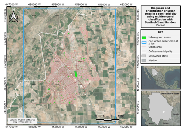
Sonora = Sonora state; Sinaloa = Sinaloa state; Durango = Durango state; Coahuila = Coahuila state; Estados Unidos de América = United States of America. Red outline = Inegi urban boundary (3 648 ha); Cyan outline = Classification area with a 2-km peri-urban buffer (17 961 ha).
Figure 1. Urban area of Delicias, Chihuahua, Mexico.
Data sources
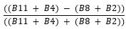
The indexes were selected to represent the biophysical processes that define the thematic classes. The summer NDVI (Normalized Difference Vegetation Index) quantifies photosynthetic activity by measuring the contrast between chlorophyll absorption in the red (B4) and the high reflectance of the mesophyll in the near-infrared (B8). ΔNDVI (Seasonal difference of NDVI) captures the phenological signal of deciduous vegetation. NDBI (Normalized Difference Built-up Index) and BSI (Bare Soil Index) leverage the high reflectance of built surfaces and mineral soil in the short-wave infrared (B11 and B12) relative to their low response in the near-infrared. The NDWI (Normalized Difference Water Index) and MNDWI (Modified Normalized Difference Water Index) identify surfaces containing water, as water is strongly absorbed in the NIR (Near-Infrared) and SWIR (Short-Wave Infrared) (Table 1). The GLCM texture metrics were calculated using band B8 because near-infrared maximizes contrast between canopy and substrate, highlighting the structural heterogeneity of the urban mosaic compared with the homogeneity of agricultural surfaces.
Table 1. Spectral indices calculated from Sentinel-2 bands.
Index |
Complete name |
Equation |
Reference |
NDVI |
Normalized Difference Vegetation Index |
|
Rouse et al. (1974) |
ΔNDVI |
Seasonal difference of NDVI |
|
— |
NDBI |
Normalized Difference Built-up Index |
|
Zha et al. (2003) |
NDWI |
Normalized Difference Water Index |
|
McFeeters (1996) |
MNDWI |
Modified Normalized Difference Water Index |
|
Xu (2006) |
BSI |
Bare Soil Index |
|
Rikimaru et al. (2002) |
B2 = Blue (492 nm); B3 = Green (560 nm); B4 = Red (665 nm); B8 = Near-infrared (NIR, 833 nm); B11 = Short-wave infrared (SWIR-1, 1 614 nm). Source: European Space Agency (ESA, 2015).
Spectral variables and classification stack
From the summer composition, six Sentinel-2 bands (B2, B3, B4, B8, B11, B12) and five indexes were extracted: NDVI, NDBI, NDWI, its modified version MNDWI and BSI, all by their acronyms in English. The winter NDVI was estimated based on the winter data, and its difference (ΔNDVI=NDVIsummer-NDVIwinter) captures the phenological signal of defoliation in deciduous walnut trees. This seasonal contrast is necessary because the distinction between evergreen and deciduous vegetation is detectable only over time: in summer, both have full foliage and similar signatures, whereas in winter, walnut defoliation creates the difference that allows them to be distinguished.
Four texture metrics derived from the grayscale co-occurrence matrix (GLCM) were also calculated (Haralick et al., 1973) across the NIR band, scaled to integers, using a 7×7-pixel (70×70 m) sliding window with averaging in four directions: contrast, correlation, energy, and entropy. The final stack included 17 variables at 10 m.
Training and validation datasets
A total of 190 polygons were digitized and classified into three categories: (1) Urban areas without vegetation (n=80: impervious surfaces and residential areas, 40 each); (2) Existing green areas (n=70; the largest number due to their internal heterogeneity: grassland, dense and scattered woodlands, ridges, and open areas); and (3) Unsuitable (n=40: walnut groves, vacant lots and agricultural land). The data were randomly split (seed=42) into 70 % for training (n=129; 99 113 pixels) and 30 % for internal validation (n=61), a split that prevents overfitting and estimates the error impartially (Maxwell et al., 2018). The independent validation (Congalton, 1991) used two references: (a) 521 GPS points from the municipal inventory, sub-pixel objects at 10 m to which a 15 m buffer was applied to ensure sufficient pixels; and (b) 290 green space polygons (88.7 ha) delineated using OpenStreetMap and visual verification (Immitzer et al., 2016). The sensitivity of (a) was evaluated at radii of 5-30 m. To include walnut groves and improve separability, the classification area was expanded with a 2-km buffer around the urban area (17 961 ha), a practice consistent with classification in urban-rural settings (Maxwell et al., 2018).
Supervised classification and accuracy evaluation
Two variants of Random Forest (Breiman, 2001) were trained in Google Earth Engine: Full RF (17 variables, 150 trees) and Reduced RF (8 variables with the highest Gini importance). Accuracy was assessed using overall accuracy, producer and consumer precision, F1-score, and the Kappa coefficient (Cohen, 1960). The hyperparameters were those of smileRandomForest (variablesPerSplit=√n; minLeafPopulation=1; bagFraction=0.5; maxNodes unlimited). The number of trees (150) was determined through sensitivity analysis (Ntree=25-300), which showed that accuracy and Kappa stabilized starting at 100 trees (variation<0.005 between 100 and 300). The reduction to 8 predictors was based on the Gini Index for the Full RF.
Assessing the deficit and prioritizing action
For the 290 polygons in the municipal inventory, the actual vegetation cover fraction was calculated through spatial matching with the RF classification (class 2 pixels). At the same time, the average land surface temperature (LST) was extracted by polygon from the Landsat-9 ST_B10 Collection 2 Level 2 thermal band (United States Geological Survey [USGS], 2024), using the official scaling factors and converting the values to degrees Celsius, at Landsat-9’s native resolution of 30 m. Prioritization was defined using decision rules based on the two variables mentioned, grouped into three levels: High (cover <25 % and LST >47 °C), Medium (cover<50 % or LST>47 °C), and Low (cover≥50 %). These thresholds are operational criteria established to translate the diagnosis into actionable categories (Figure 2). Improving green infrastructure under this approach is consistent with the strategy of gradual intervention by Wolch et al. (2014).
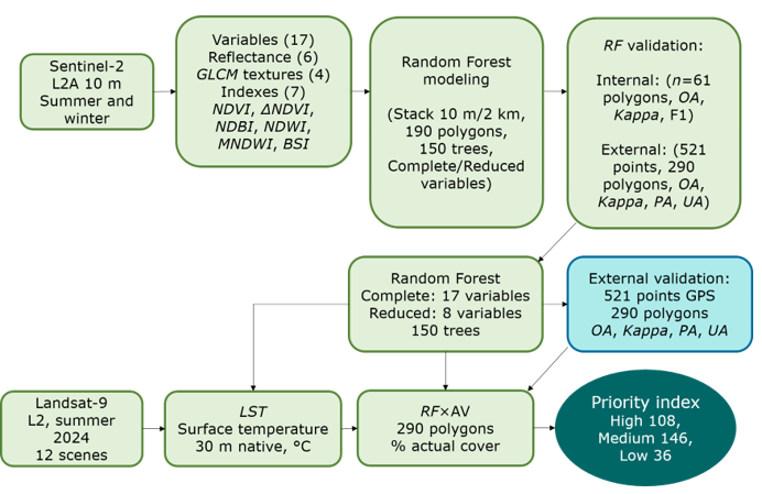
RF = Random Forest; LST = Land surface temperature. GLCM = Gray-level co-occurrence matrix; AV = Urban green areas; OA = Overall accuracy; PA = Producer’s accuracy; UA = User’s accuracy; L2A = Level 2A (Sentinel-2 processing level); L2 = Collection 2 Level 2 (Landsat). The dotted line indicates the flow of supplementary thermal data.
Figure 2. Flowchart of the methodological process.
Results
Significance of variables
The contrast GLCM texture (3 609) and the SWIR bands (B12=3 528; B11=3 301) showed the highest relative importance, followed by texture correlation (3 292), while the winter NDVI (3 221) and ΔNDVI (3 098) indexes occupied intermediate positions in relative importance, providing the signal of deciduous seasonality in walnut groves that complements the texture and short-wave infrared variables (Figure 3). TEX_entropy (2 120) and TEX_energy (2 437) had the lowest contributions and were excluded from the Reduced RF.
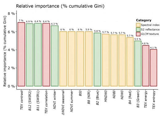
Horizontal bars sorted by importance and colored by category.
Figure 3. Relative importance of the 17 variables in the classification stack (cumulative Gini impurity index).
Accuracy of classification models
The Complete RF achieved an overall accuracy of 89.1 % and a Kappa coefficient of 0.662, indicating substantial agreement (Table 2). The Reduced RF (8 variables) showed equivalent results (accuracy=89.0 %, Kappa=0.658), confirming that the parsimonious model is equally suitable for this context. The confusion matrix (Table 3) reveals that the main source of error was confusion between Existing green and Unsuitable (2 149 misclassified pixels out of a total of 2 543), attributable to the small size of the urban parks and spectral overlap between low-density perennial vegetation and walnut groves during the phenological transition period. Independent validation using the 521 municipal GPS points yielded a producer accuracy of 18.0 % for Existing green areas. The sensitivity analysis of the buffer radius showed a monotonic decrease in this metric as the radius increased (21.4 %, 20.2 %, 18.0 %, 17.2 %, and 14.5 % for 5, 10, 15, 20, and 30 m, respectively), confirming the inclusion of impermeable perimeter pixels. However, even at the minimum radius, accuracy remained below 22 percent; therefore, this parameter cannot explain the low detection rate, which instead reflects the absence of functional vegetation cover at most surveyed sites.
Table 2. Accuracy comparison—internal validation (70/30 split, n=61 ROIs).
Model |
Kappa |
Global accuracy |
Observations |
Full RF (17 variables) |
0.662 |
89.1 % |
Selected model |
Reduced RF (8 variables) |
0.658 |
89.0 % |
A more parsimonious model |
ROI = Regions of interest; reference polygons used for classifier training and validation.
Table 3. Full RF confusion matrix.
Actual Predicted class |
Urban |
Green |
Unsuitable |
Actual total |
Urban without vegetation |
4 029 |
78 |
836 |
4 943 |
Existing green space |
164 |
230 |
2 149 |
2 543 |
Unsuitable |
283 |
11 |
24 791 |
25 085 |
Predicted total |
4 476 |
319 |
27 776 |
32 571 |
Spectral separability between classes
The three classes differed significantly across the four variables (Kruskal-Wallis test, p<0.005; Table 4, Figure 4), although their discriminatory power varied. Summer NDVI was the most discriminating variable (ε²=0.438) and the only one that distinguished the three classes (Dunn, p<0.05), with a gradient ranging from 0.111 in Urban without vegetation to 0.360 in Existing green. Texture entropy distinguished Unsuitable from the other classes (p<0.001), but did not differentiate Urban without vegetation from Existing green space. ΔNDVI distinguished urban green areas (0.062) from impervious surfaces (0.003), but not from Unsuitable (0.066; p=0.390), and LST did not distinguish between the two vegetated classes (p=1.000). This limitation reflects the bimodal composition of the Unsuitable category, which groups deciduous walnut groves with vacant lots and agricultural land.
Table 4. Comparison of spectral, thermal, and texture variables among the three thematic classes using the Kruskal-Wallis test.
Variable |
Urban without vegetation (n=80) |
Existing green areas (n=70) |
Unsuitable (n=40) |
H |
p |
ε² |
Effect |
NDVIsummer |
0.111± 0.096a |
0.360± 0.142b |
0.290± 0.237c |
84.0 |
<0.001 |
0.438 |
Large |
ΔNDVI |
0.003± 0.042a |
0.062± 0.081b |
0.066± 0.133ab |
19.0 |
<0.001 |
0.091 |
Moderate |
LST (°C) |
48.0± 2.01a |
46.9± 1.40b |
45.8± 4.43b |
10.8 |
0.005 |
0.047 |
Small |
Textural entropy |
4.291± 0.017a |
4.291± 0.016a |
4.281± 0.012b |
21.9 |
<0.001 |
0.106 |
Moderate |
Mean±standard deviation of the mean values by ROI polygon. H = Kruskal-Wallis statistic (df=2); ε² = Effect size. Different letters within the same row indicate significant differences between classes (Dunn's test with Bonferroni correction, p<0.05); classes sharing the same letter do not differ significantly.
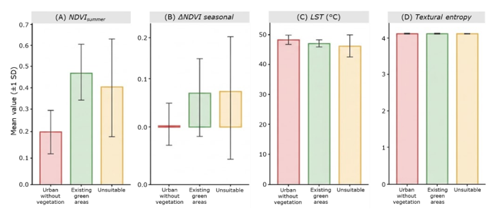
A = Summer NDVI; B = Seasonal ΔNDVI; C = LST (°C); D = Textural entropy. The error bars represent ±1 standard deviation (SD).
Figure 4. Average value by class.
Classified land area and green cover assessment
The Full RF’s classification within the consolidated urban area (3 643.6 ha) reveals a marked predominance of impervious surfaces and a significantly reduced amount of green space, with barely 7.17 m2 per inhabitant. It also highlights that more than a quarter of the urban area consists of walnut orchards and peri-urban agricultural land, underscoring the challenge of spectral separability inherent in this type of semi-arid agricultural city (Table 5).
Table 5. Area classified by thematic class-Full RF (Sentinel-2 10 m, INEGI, 2020 boundaries).
Class |
Surface area (ha) |
Proportion (%) |
m2 inhab-1 |
Urban without vegetation |
2 591.3 |
71.0 |
— |
Existing green areas |
107.9 |
3.0 |
7.17 |
Unsuitable (walnut orchards/agricultural) |
944.4 |
25.9 |
— |
Total urban area |
3 643.6 |
100.0 |
— |
Spatial overlay of the classification data with the 290 polygons in the municipal inventory revealed a substantial discrepancy: of the 88.7 ha recorded as green areas, only 21.8 ha (24.6 %) have functional vegetation detectable at a distance of 10 m. More than one-third of that area (33.2 ha; 37.4 %) consists of impervious soil, and a similar proportion (33.5 ha; 37.7 %) consists of walnut orchards and peri-urban farmland (Table 6; Figure 5).
Table 6. Full RF spatial overlap×municipal inventory (290 polygons, 88.7 ha).
RF class within nominal GAs |
Surface area (ha) |
% of the nominal GAs |
Existing green areas |
21.8 |
24.6 % |
Urban without vegetation |
33.2 |
37.4 % |
Unsuitable |
33.5 |
37.7 % |
Nominal total |
88.7 |
100.0 % |
GAs = Green areas. The sum does not equal the total due to unclassified edge pixels.
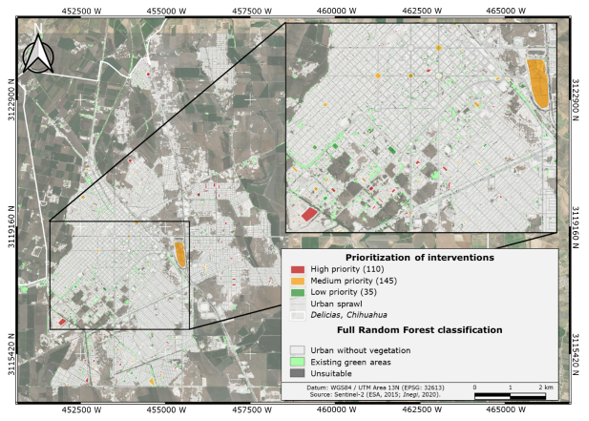
Figure 5. Random Forest Classification and intervention priority levels in Delicias, Chihuahua, Mexico.
This gap is not distributed evenly across the surveyed areas. By polygon, the distribution is concentrated in the lower coverage ranges: 122 of the 290 areas (42.1 %) have less than 5 % detected vegetation, and only a minority exceed 50 %. The municipal inventory therefore does not distinguish between the administrative zone and the vegetation it is supposed to contain: a considerable portion of spaces classified as green areas lacks functional tree or herbaceous cover. Of the 290 registered sites, 122 (42.1 %) have less than 5 % detected vegetation cover, and only 81 (27.9 %) exceed 50 %, confirming that many cataloged green areas lack functional vegetation cover.
Priority for action in existing green spaces
The Priority index (based on RF coverage deficit and average LST) classified the 290 green spaces into three urgency levels (Figure 5; Table 7). The 110 high-priority areas (first line of municipal action) have only 4.4 % actual coverage and an LST>47 °C, indicating severe heat stress and a complete lack of functional vegetation. Overall, the inventory shows a deficit of 67.1 ha without detectable vegetation (4.46 m2 per inhabitant), officially classified as green areas that do not fulfill that function.
Table 7. Priority for tree maintenance in green spaces listed in the municipal inventory (290 polygons).
Priority |
Polygons |
Nominal Surface area (ha) |
Actual RF green areas (ha) |
Deficit (ha) |
Criterion |
High |
110 |
31.0 |
1.4 |
29.6 |
<25 % and LST>47°C |
Medium |
145 |
47.8 |
12.4 |
35.4 |
<50 % or LST>47°C |
Low |
35 |
10.3 |
8.0 |
2.3 |
≥50 % cover RF |
Overall |
290 |
88.7 |
21.8 |
67.2 |
4.46 m² hab⁻¹ |
Discussion
Classifier performance and the role of seasonal ΔNDVI
The model achieved a Kappa coefficient of 0.662, indicating substantial agreement consistent with the range (0.58-0.78) reported for complex classifications using Sentinel-2 and machine learning (Immitzer et al., 2016; Maxwell et al., 2018). Accuracy relies primarily on GLCM contrast texture and the SWIR bands (B12, B11), which distinguish mineral substrate from vegetation canopy. The marginal difference between the Full and Reduced RF (ΔKappa=0.004) confirms that the nine excluded variables provide redundant information, and that the parsimonious model promotes efficiency in recurring monitoring (Maxwell et al., 2018; Zhao et al., 2024).
The absence of significant differences in ΔNDVI between Existing green areas and Unsuitable (Table 4) does not reflect a limitation of the index, but rather the heterogeneous composition of the latter class. A subsequent diagnostic analysis showed that the ΔNDVI for walnut groves (0.269±0.138) differs significantly from that of urban evergreen trees (0.062±0.081; Dunn, p=0.002), while vacant lots have values close to zero (0.023±0.085). The overlap between the aggregated class mean (0.066) and that of Existing green vegetation, therefore, results from combining two subpopulations with opposite phenological behaviors. ΔNDVI distinguishes between deciduous and evergreen vegetation; the limitation lies in applying measures of central tendency to bimodal classes (Hartigan & Hartigan, 1985).
Discrepancy between nominal inventory and actual vegetation cover
The most significant finding is the discrepancy between the official records and satellite data: only 24.6 % of the 88.7 ha classified as green areas contain functional vegetation, while 37.4 % consists of impervious surfaces. This overestimation occurs because traditional inventories delineate entire administrative districts, including paved plazas, concrete roundabouts, and parking lots without trees, as confirmed by the producer’s low accuracy rate of 18.0 % during validation against the official dataset. It is imperative to redefine public green infrastructure by establishing a minimum threshold for detectable tree cover to classify a plot as a true green area; this threshold, which can be calibrated according to the sensor and local standards, serves as a replicable tool for satellite monitoring in similar cities (Shahtahmassebi et al., 2021).
Lack of tree cover and public policy
The assessed coverage is only 7.17 m2 per inhabitant. Compared with the UN-Habitat benchmark of 9.0 m2 per inhabitant, SDG 11 and the New Urban Agenda offer a more robust framework focused on equitable accessibility and ecosystem services rather than a single threshold (Borelli et al., 2018). To overcome the deficit (1.83 m2 per inhabitant), approximately 27.5 ha would need to be developed; the most viable strategy is not to acquire new land, but rather to intervene in the 110 high-priority areas (95.6 % of which have no detectable vegetation), capitalizing on existing infrastructure and promoting functional spaces (Wolch et al., 2014). The 67.1 ha shortfall, areas already classified as green spaces but lacking any functional purpose (4.46 m2 per inhabitant), is the central empirical argument for reforming the greening policy.
Surface temperature and the urban cold island effect
The thermal gradient exhibited a distinctive pattern: surfaces without vegetation (48.0 °C), urban green spaces (46.9 °C), and unsuitable areas (45.8 °C). The fact that the canopy of walnut groves provides more cooling than the few urban parks is due to the continuity of agricultural land and constant irrigation, which maximize evapotranspiration, a “cool island or urban oasis” effect documented in compact, arid cities, which is the opposite of the heat island effect found in temperate cities (Jáuregui, 1993; Villanueva-Solis et al., 2013). Given that increased vegetation cover consistently reduces surface temperature in urban environments (Bowler et al., 2010), with mitigations on the order of ~1.1 °C documented in desert cities in Northern Mexico (López-González et al., 2021), planting trees in the 110 high priority polygons (30.7 ha) would significantly mitigate local thermal stress.
Limitations of the study and future research
A resolution of 10 m is insufficient to detect individual trees on medians or sidewalks, which points to the use of higher-resolution imagery (PlanetScope, WorldView) as a future line of work; the sensor’s resolution substantially affects coverage estimates and their comparability (Wu et al., 2023). Prioritization was based on rules with operational thresholds that could be improved through multi-criteria calibration with local managers. Finally, the GPS validation inventory was not designed to validate satellite products, as it lacks data on the fraction of coverage as a rigorous reference (Congalton, 1991). Although the results pertain to Delicias, the approach is transferable to medium-sized cities in semi-arid regions with peri-urban deciduous agriculture, as it uses freely available inputs and does not require farmland and can therefore be easily replicated by local governments with limited resources.
Conclusions
Multitemporal classification using Random Forest on Sentinel-2 data enabled the identification of urban green space in a semi-arid city with deciduous peri-urban vegetation (accuracy 89.1 %, Kappa=0.662). Summer NDVI was the most discriminating variable, while seasonal ΔNDVI distinguished deciduous from evergreen vegetation—a distinction that single-time-step approaches cannot achieve and that applies to agricultural cities in the arid North. Cross-validation confirmed a systematic overestimation of the municipal inventory: only 24.6 % of the 88.7 ha recorded show detectable vegetation cover, and a mere 3.0 % of the urban area consists of functional vegetation (7.17 m2 per inhabitant). Traditional land-use records do not distinguish between the administrative district and the vegetation it should contain —a discrepancy satellite auditing can quantify. Intervention zoning provides a spatially explicit and replicable criterion for directing municipal investment toward areas with the greatest thermal and vegetation deficits, in line with SDG 11. However, this exploratory, rule-based approach can be calibrated collaboratively. Notable limitations include a 10 m resolution, digitization without field verification, and non-proportional sample allocation. The findings support the need to establish verifiable tree-cover thresholds for registering green spaces, laying the groundwork for auditing municipal inventories with remote sensing.
Acknowledgments
The authors are grateful to Óscar Jiménez Azpeitia, Engineer and Head of the Environment Department of the Delicias municipality, Chihuahua, for providing the georeferenced inventory of green areas.
Conflict of interest
The authors declare that they have no conflict of interest.
Contribution by author
Samuel Alberto García-García and Ana Marissa de la Fuente-Solís: conceptualization and methodological design, data processing, analysis of results, and drafting of the manuscript; Joel Rascón-Solano: statistical analysis; Luisa Patricia Uranga-Valencia: critical review and editorial guidance; Rufino Sandoval-García: data processing, analysis, and validation of results.
References
Belgiu, M., & Drăguţ, L. (2016). Random forest in remote sensing: A review of applications and future directions. ISPRS Journal of Photogrammetry and Remote Sensing, 114, 24-31. https://doi.org/10.1016/j.isprsjprs.2016.01.011
Borelli, S., Conigliaro, M., & Pineda, F. (2018). Los bosques urbanos en el contexto global. Unasylva: Revista Internacional de Silvicultura e Industrias Forestales, 69(250), 3-10. https://dialnet.unirioja.es/servlet/articulo?codigo=7455599
Bowler, D. E., Buyung-Ali, L., Knight, T. M., & Pullin, A. S. (2010). Urban greening to cool towns and cities: A systematic review of the empirical evidence. Landscape and Urban Planning, 97(3), 147-155. https://doi.org/10.1016/j.landurbplan.2010.05.006
Breiman, L. (2001). Random forests. Machine Learning, 45, 5-32. https://doi.org/10.1023/A:1010933404324
Cohen, J. (1960). A coefficient of agreement for nominal scales. Educational and Psychological Measurement, 20(1), 37-46. https://doi.org/10.1177/001316446002000104
Congalton, R. G. (1991). A review of assessing the accuracy of classifications of remotely sensed data. Remote Sensing of Environment, 37(1), 35-46. https://doi.org/10.1016/0034-4257(91)90048-B
Cuervo-Robayo, A. P., Téllez-Valdés, O., Gómez-Albores, M. A., Venegas-Barrera, C. S., Manjarrez, J., & Martínez-Meyer, E. (2013). An update of high-resolution monthly climate surfaces for Mexico. International Journal of Climatology, 34(7), 2427-2437. https://doi.org/10.1002/joc.3848
Dobbs, C., Escobedo, F. J., & Zipperer, W. C. (2011). A framework for developing urban forest ecosystem services and goods indicators. Landscape and Urban Planning, 99(3-4), 196-206. https://doi.org/10.1016/j.landurbplan.2010.11.004
European Space Agency. (2015). Sentinel-2 user handbook (Issue 1, Rev. 2). European Space Agency. https://sentinels.copernicus.eu/documents/247904/685211/Sentinel-2_User_Handbook
García, E. (1973). Modificaciones al sistema de clasificación climática de Köppen (2da ed.). Instituto de Geografía, Universidad Nacional Autónoma de México. https://publicaciones.geografia.unam.mx/index.php/ig/catalog/book/83
Gorelick, N., Hancher, M., Dixon, M., Ilyushchenko, S., Thau, D., & Moore, R. (2017). Google Earth Engine: Planetary-scale geospatial analysis for everyone. Remote Sensing of Environment, 202, 18-27. https://doi.org/10.1016/j.rse.2017.06.031
Haralick, R. M., Shanmugam, K., & Dinstein, I. (1973). Textural features for image classification. IEEE Transactions on Systems, Man, and Cybernetics, 3(6), 610-621. https://doi.org/10.1109/TSMC.1973.4309314
Hartigan, J. A., & Hartigan, P. M. (1985). The dip test of unimodality. The Annals of Statistics, 13(1), 70-84. https://www.jstor.org/stable/2241144
Immitzer, M., Vuolo, F., & Atzberger, C. (2016). First experience with Sentinel-2 data for crop and tree species classifications in central Europe. Remote Sensing, 8(3), Article 166. https://doi.org/10.3390/rs8030166
Instituto Nacional de Estadística y Geografía. (2020). Censo de Población y Vivienda 2020 (Base de datos). Instituto Nacional de Estadística y Geografía. https://www.inegi.org.mx
Jáuregui, E. (1993). Mexico City's urban heat island revisited. Erdkunde, 47(3), 185-195. https://doi.org/10.3112/erdkunde.1993.03.03
Livesley, S. J., McPherson, E. G., & Calfapietra, C. (2016). The urban forest and ecosystem services: impacts on urban water, heat, and pollution cycles at the tree, street, and city scale. Journal of Environmental Quality, 45(1), 119-124. https://doi.org/10.2134/jeq2015.11.0567
López-González, F. M., Navarro-Navarro, L. A., Díaz-Caravantes, R. E., & Navarro-Estupiñán, J. (2021). Cobertura vegetal y la distribución de islas de calor/oasis urbanos en Hermosillo, Sonora. Frontera Norte, 33, Artículo 6. https://doi.org/10.33679/RFN.V1I1.2088
Manzanilla-Quiñones, U., Manzanilla-Quijada, G. E., & Delgado-Valerio, P. (2021). Análisis espacio-temporal de las áreas verdes urbanas de la Zona Metropolitana de Monterrey, México. Ecosistemas y Recursos Agropecuarios, 8(1). https://doi.org/10.19136/era.a8n1.2676
Maxwell, A. E., Warner, T. A., & Fang, F. (2018). Implementation of machine-learning classification in remote sensing: an applied review. International Journal of Remote Sensing, 39(9), 2784-2817. https://doi.org/10.1080/01431161.2018.1433343
McFeeters, S. K. (1996). The use of the Normalized Difference Water Index (NDWI) in the delineation of open water features. International Journal of Remote Sensing, 17, 1425-1432. https://doi.org/10.1080/01431169608948714
Rikimaru, A., Roy, P. S., & Miyatake, S. (2002). Tropical forest cover density mapping. Tropical Ecology, 43(1), 39-47. https://www.researchgate.net/publication/255718070_Tropical_forest_cover_density_mapping
Rodriguez-Galiano, V. F., Ghimire, B., Rogan, J., Chica-Olmo, M., & Rigol-Sanchez, J. P. (2012). An assessment of the effectiveness of a random forest classifier for land-cover classification. ISPRS Journal of Photogrammetry and Remote Sensing, 67, 93-104. https://doi.org/10.1016/j.isprsjprs.2011.11.002
Rouse, Jr., J. W., Haas, R. H., Schell, J. A., Deering, D. W., & Harlan, J. C. (1974). Monitoring the vernal advancement and retrogradation (greenwave effect) of natural vegetation (No. E75-10354). Texas A&M University. https://ntrs.nasa.gov/api/citations/19750020419/downloads/19750020419.pdf
United States Geological Survey. (2024, May 23). Landsat 8-9 Collection 2 Level 2 Science Product Guide [LSDS-1619, Version 6.0]. United States Geological Survey. https://d9-wret.s3.us-west-2.amazonaws.com/assets/palladium/production/s3fs-public/media/files/LSDS-1619_Landsat8-9-Collection2-Level2-Science-Product-Guide-v6.pdf
Servicio de Información Agroalimentaria y Pesquera. (2024). Cierre de la producción agrícola por estado y municipio (Base de datos). Gobierno de México. https://nube.agricultura.gob.mx/cierre_agricola/
Shahtahmassebi, A. R., Li, C., Fan, Y., Wu, Y., Lin, Y., Gan, M., Wang, K., Malik, A., & Blackburn, G. A. (2021). Remote sensing of urban green spaces: A review. Urban Forestry & Urban Greening, 57, Article 126946. https://doi.org/10.1016/j.ufug.2020.126946
Villanueva-Solis, J., Ranfla, A., & Quintanilla-Montoya, A. L. (2013). Isla de Calor Urbana: modelación dinámica y evaluación de medidas de mitigación en ciudades de clima árido extremo. Información Tecnológica, 24(1), 15-24. https://doi.org/10.4067/S0718-07642013000100003
Wolch, J. R., Byrne, J., & Newell, J. P. (2014). Urban green space, public health, and environmental justice: The challenge of making cities ‘just green enough’. Landscape and Urban Planning, 125, 234-244. https://doi.org/10.1016/j.landurbplan.2014.01.017
Wu, S., Yu, W., An, J., Lin, C., & Chen, B. (2023). Remote sensing of urban greenspace exposure and equality: Scaling effects from greenspace and population mapping. Urban Forestry & Urban Greening, 90, Article 128136. https://doi.org/10.1016/j.ufug.2023.128136
Xu, H. (2006). Modification of normalised difference water index (NDWI) to enhance open water features in remotely sensed imagery. International Journal of Remote Sensing, 27(14), 3025-3033. https://doi.org/10.1080/01431160600589179
Zha, Y., Gao, J., & Ni, S. (2003). Use of normalized difference built-up index in automatically mapping urban areas from TM imagery. International Journal of Remote Sensing, 24, 583-594. https://doi.org/10.1080/01431160304987
Zhao, Z., Islam, F., Waseem, L. A., Tariq, A., Nawaz, M., Islam, I. U., Bibi, T., Rehman, N. U., Ahmad, W., Aslam, R. W., Raza, D., & Hatamleh, W. A. (2024). Comparison of three machine learning algorithms using Google Earth Engine for land use land cover classification. Rangeland Ecology & Management, 92, 129-137. https://doi.org/10.1016/j.rama.2023.10.007
Zhou, W., Cadenasso, M. L., Schwarz, K., & Pickett, S. T. A. (2014). Quantifying spatial heterogeneity in urban landscapes: integrating visual interpretation and object-based classification. Remote Sensing, 6(4), 3369-3386. https://doi.org/10.3390/rs6043369
Todos los textos publicados por la Revista Mexicana de Ciencias Forestales –sin excepción– se distribuyen amparados bajo la licencia Creative Commons 4.0 Atribución-No Comercial (CC BY-NC 4.0 Internacional), que permite a terceros utilizar lo publicado siempre que mencionen la autoría del trabajo y a la primera publicación en esta revista.